Buffy

Sorts MC sensors info into buffers, slays vampires, etc

Full simulations generate sensor (PMTs and SiPMs) responses, including the time and the detected charge of a specific signal. However, this sensor information does not have the waveform format obtained from the detector. Buffy takes nexus sensors’ information, and sorts it into true waveforms (TWF). TWFs represent the signal amplitude of a given sensor without any type of distortion or effect from the electronics within a certain time interval given by the sensor sampling time. This type of time ordering of the sensor signal in a data-like format is what is called bufferisation. TWFs generated by Buffy can be transformed into raw waveforms RWFs (i.e. with effects from the electronics) with Diomira. For detector geometries without sensor electronics, a simplified electronics modeling can be applied with Hypathia to transform TWFs directly into PMaps.

Input

• /MC/hits

• /MC/particles

• /MC/sns_response

Output

• /Run/runInfo: run info table

• /Run/events: event info table

• /Run/eventMap: table that connects event id and nexus event numbering

• /RD/pmtrd/: time ordered signal amplitude of the PMTs in true photoelectrons (PMT buffers). array with shape: (number of events, number of PMTs, length of PMT waveform)

• /RD/sipmrd/: time ordered signal amplitude of the SiPMs in true photoelectrons (SiPM buffers). array with shape: (number of events, number of SiPMs, length of SiPM waveform).

Config

Besides the Common arguments to every city, Buffy has the following arguments:

Parameter	Type	Description
max_time	float	Maximum duration of the event that will be taken into account starting from the first detected signal. All signals after that are lost. Must be greater than buffer_length. If not, raises a warning and sets max_time == buffer_length. It should be a multiple of 1 \(\mu s\).
buffer_length	float	Configured buffer length in \(\mu s\).
pre_trigger	float	Time in buffer before identified signal in \(\mu s\).
trigger_threshold	int	Trigger threshold for selection in \(pe\)s.

Workflow

For full simulations, NEXUS /MC/sns_response table stores for each event (event_id) the list of sensors (sensor_id) that detect a specific number of photons (charge) in an ordered number of the time bin (time_bin).

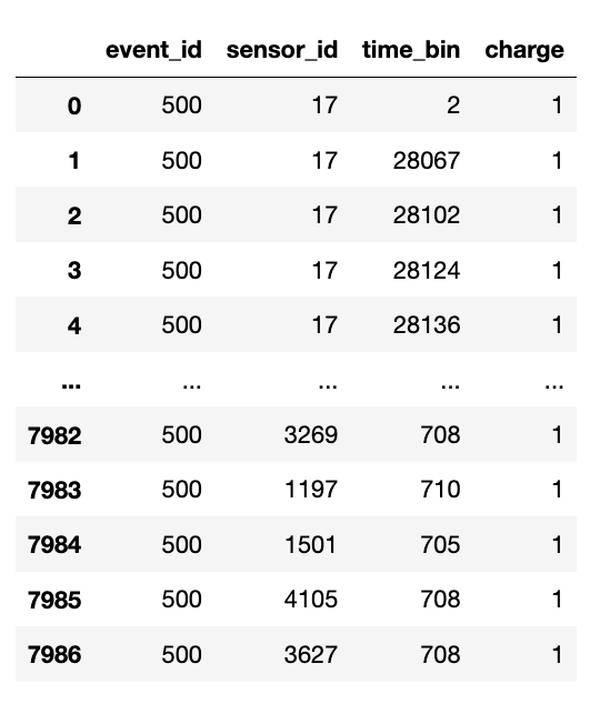
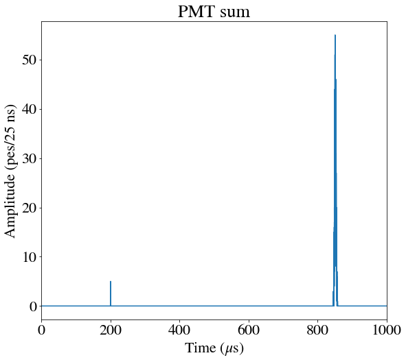
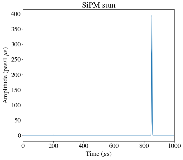
More details about nexus output can be found in its Github Wiki . This type of tables do not have the same shape that the waveforms collected when data taken, and in addition they only provide the information from the sensors and time bins when some charge is detected. Buffy takes this information (event_id, sensor_id and time_bin), and transforms it into the waveform shape of the TWF expected for each type of sensor: pmtrd and sipmtrd (PMTs and SiPMs respectively) based on the bufferisation parameters provided. Pictures below represent the output for PMTs and SiPMs waveforms.

This process is separated in the following tasks in the city:

• Histogram creation

• Signal Search

• Synchronisation and trigger separation

Buffy output also includes /Run/runInfo and /Run/events tables as the ones generated during data taking.

Note

Historically, Buffy is based in an initial code of detsim (https://github.com/next-exp/IC/tree/master/invisible_cities/detsim) and most of its functions are located in that path but they are independent to Detsim city.

Histogram creation

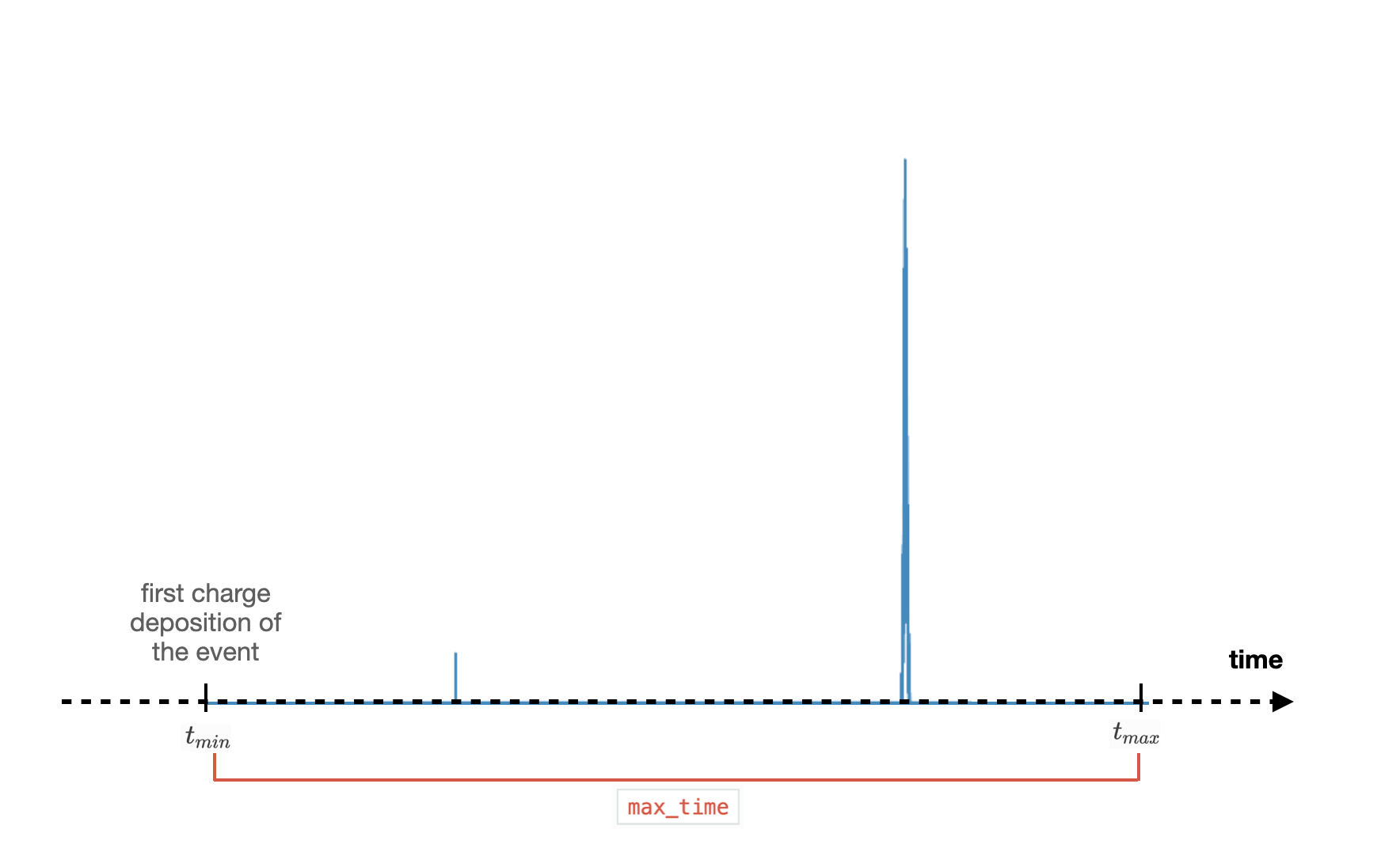
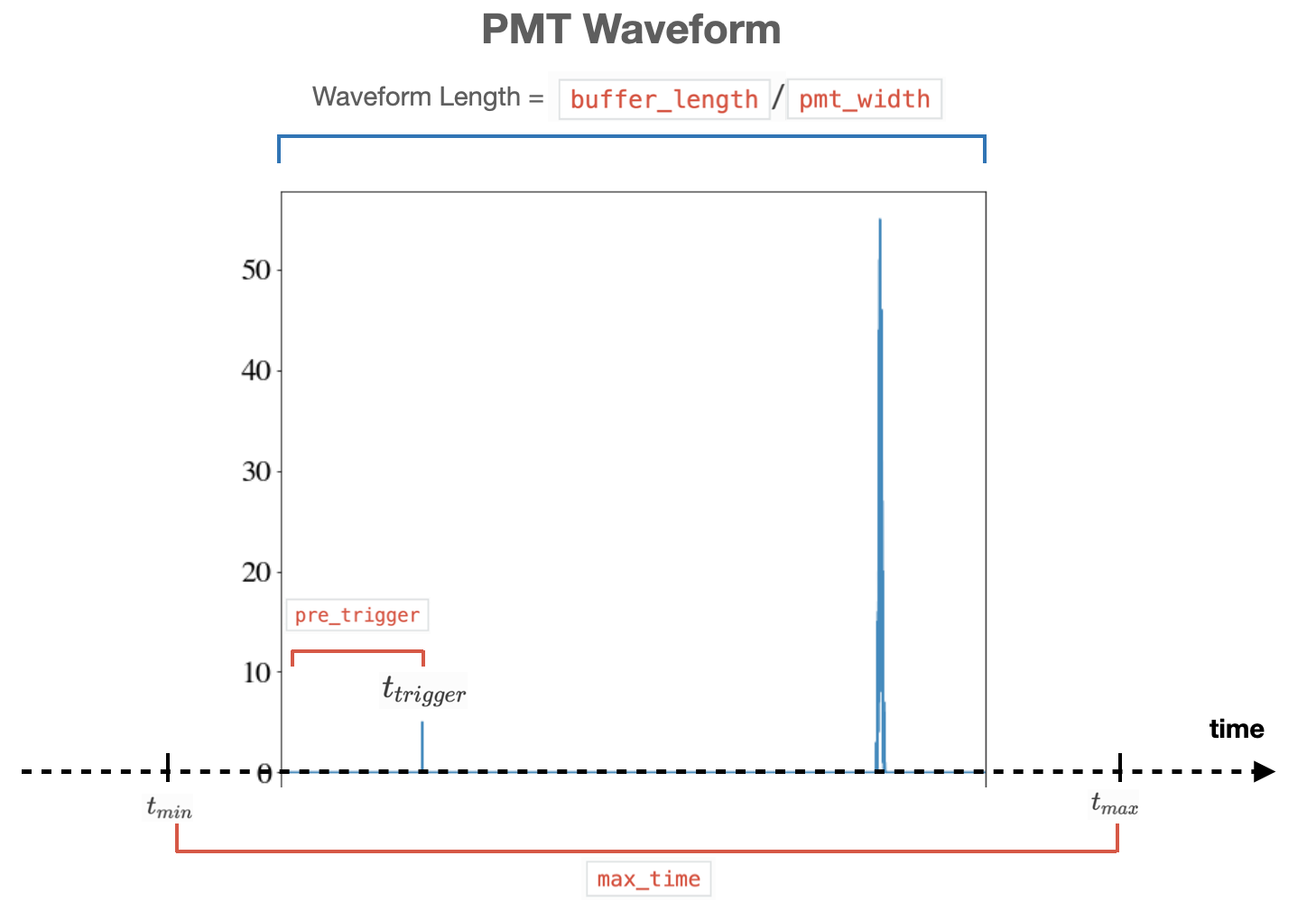
As it was highlighted earlier, NEXUS information about sensor hits (/MC/sns_response) comes binned in time based on when a sensor sees some energy deposition. This means that the time_bin column numbers are increasing for a given event, but they can have gaps since empty time bins are not stored. This initial part of the city checks the time stamp of an event according to the sensors’ response and defines histograms of charge distribution between [\(t_{min}\), \(t_{max}\)], being:

• \(t_{min}\): the time stamp of the first charge deposition of the event,

• \(t_{max}\): defined considering that max_time = \(t_{max}\) - \(t_{min}\).

These histograms (one for PMTs and another for SiPMs) are defined by summing all individual sensors. This step restores also empty bins by padding zeros in between separate signals, and sample the histograms according to the binning of each type of sensor (pmt_width and sipm_width). Sampling widths are included in the simulation parameters (/MC/configuration), and depend on the type of sensor and detector. Normally correspond to 25 \(ns\) for PMTs and and 1 \(\mu s\) for SiPMs.

Signal Search

Once the charge is distributed in the previously defined histograms, the code searches for signal-like events. It takes the PMT sum histogram and looks for the first value of the binned charge above a certain threshold (trigger_threshold), and defines the trigger time, \(t_{trigger}\). Waveforms are therefore defined for PMTs:

• shifting the times of the charge histogram such that the first value over threshold (\(t_{trigger}\)) falls at the time defined as pre_trigger;

• setting the length (in number of samples) as requested in the config parameters (buffer_length/pmt_width).

Note

\(t_{min}\) does not need to be at 0, since it is defined based on the first charge deposition, independently if it is above the trigger_threshold or not.

Synchronisation and trigger separation

Since the buffer length is different for PMTs and SiPMs, it is necessary to align and synchronise the signals between waveforms. Waveforms are then sliced according to binning (pmt_width and sipm_width), trigger time and configured pre-trigger (pre_trigger). Once PMT sum and SiPM sum waveforms are synchronised, individual sensor waveforms are generated. If more than one trigger is found separated from each other by more than a buffer width, the nexus event can be split into multiple data-like waveforms.